NO.PZ201709270100000502
问题如下:
Max Busse is an analyst in the research department of a large hedge fund. He was recently asked to develop a model to predict the future exchange rate between two currencies. Busse gathers monthly exchange rate data from the most recent 10-year period and runs a regression based on the following AR(1) model specification:
Regression 1: xt = b0 + b1xt–1 + εt, where xt is the exchange rate at time t.
Based on his analysis of the time series and the regression results, Busse reaches the following conclusions:
Conclusion 1: The variance of xt increases over time.
Conclusion 2: The mean-reverting level is undefined.
Conclusion 3: b0 does not appear to be significantly different from 0.
Busse decides to do additional analysis by first-differencing the data and running a new regression.
Regression 2: yt = b0 + b1yt–1 + εt, where yt = xt – xt–1.
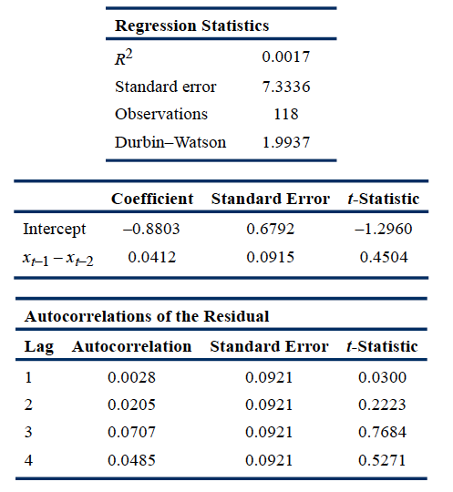
Exhibit 1 shows the regression results.
Exhibit 1. First-Differenced Exchange Rate AR(1) Model: Month-End Observations, Last 10 Years

Note: The critical t-statistic at the 5% significance level is 1.98.
Busse decides that he will need to test the data for nonstationarity using a Dickey–Fuller test. To do so, he knows he must model a transformed version of Regression 1. Busse’s next assignment is to develop a model to predict future quarterly sales for PoweredUP, Inc., a major electronics retailer. He begins by running the following regression:
Regression 3: ln Salest – ln Salest–1 = b0 + b1(ln Salest–1 – ln Salest–2) + εt.
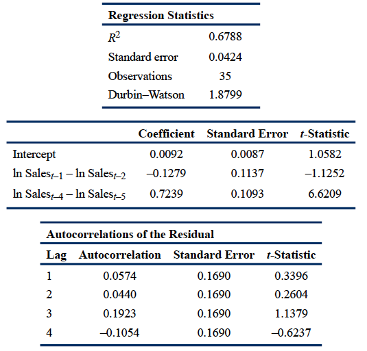
Exhibit 2 presents the results of this regression.
Exhibit 2. Log Differenced Sales: AR(1) Model PoweredUP, Inc., Last 10 Years of Quarterly Sales

Note: The critical t-statistic at the 5% significance level is 2.02.
Because the regression output from Exhibit 2 raises some concerns, Busse runs a different regression. These regression results, along with quarterly sales data for the past five quarters, are presented in Exhibits 3 and 4, respectively.
Exhibit 3. Log Differenced Sales: AR(1) Model with Seasonal Lag PoweredUP, Inc., Last 10 Years of Quarterly Sales

Note: The critical t-statistic at the 5% significance level is 2.03.
Exhibit 4. Most Recent Quarterly Sales Data (in billions)

After completing his work on PoweredUP, Busse is asked to analyze the relationship of oil prices and the stock prices of three transportation companies. His firm wants to know whether the stock prices can be predicted by the price of oil. Exhibit 5 shows selected information from the results of his analysis.
Exhibit 5. Analysis Summary of Stock Prices for Three Transportation Stocks and the Price of Oil

To assess the relationship between oil prices and stock prices, Busse runs three regressions using the time series of each company’s stock prices as the dependent variable and the time series of oil prices as the independent variable.
2. Based on the regression output in Exhibit 1, the first-differenced series used to run Regression 2 is consistent with:
选项:
A.a random walk.
B.covariance stationarity.
C.a random walk with drift.
解释:
B is correct. The critical t-statistic at a 5% confidence level is 1.98. As a result, neither the intercept nor the coefficient on the first lag of the first-differenced exchange rate in Regression 2 differs significantly from zero. Also, the residual autocorrelations do not differ significantly from zero. As a result, Regression 2 can be reduced to yt = εt with a mean-reverting level of b0/(1 – b1) = 0/1 = 0.
Therefore, the variance of yt in each period is Var(εt) = σ2. The fact that the residuals are not autocorrelated is consistent with the covariance of the times series, with itself being constant and finite at different lags. Because the variance and the mean of yt are constant and finite in each period, we can also conclude that yt is covariance stationary.
因为因变量是yt-yt-1,这里验证的应该是g=0,也就是covaraince non stationary?


